| 일 | 월 | 화 | 수 | 목 | 금 | 토 |
|---|---|---|---|---|---|---|
| 1 | 2 | 3 | ||||
| 4 | 5 | 6 | 7 | 8 | 9 | 10 |
| 11 | 12 | 13 | 14 | 15 | 16 | 17 |
| 18 | 19 | 20 | 21 | 22 | 23 | 24 |
| 25 | 26 | 27 | 28 | 29 | 30 | 31 |
- cl
- NLP #자연어 처리 #CS224N #연세대학교 인공지능학회
- cv
- YAI 10기
- CS224N
- RCNN
- 강화학습
- YAI 11기
- nerf
- YAI 8기
- 컴퓨터 비전
- 연세대학교 인공지능학회
- CS231n
- GAN #StyleCLIP #YAI 11기 #연세대학교 인공지능학회
- VIT
- PytorchZeroToAll
- YAI 9기
- Googlenet
- GaN
- Faster RCNN
- rl
- Fast RCNN
- 자연어처리
- 컴퓨터비전
- transformer
- NLP
- 3D
- YAI
- Perception 강의
- CNN
- Today
- Total
연세대 인공지능학회 YAI
[논문 리뷰] Diffusion Models Beat GANs on Image Synthesis 본문
Diffusion Models Beat GANs on Image Synthesis
** YAI 9기 최성범님께서 DIffusion팀에서 작성한 글입니다.
Abstract
- Generation model중 diffusion models이 SOTA를 달성
- 이를 위해 better architecture와 classifier guidance를 사용함
- Classifier guidance는 classifier의 gradients를 사용하고, generated image의 diversity와 fidelity의 trade off 관계가 있음
1. Introduction
GAN은 최근 FID, Inception Score, Precision metric으로 측정한 image generation task에서 SOTA를 달성했다. 그러나 이러한 metric은 생성한 이미지 측면의 다양성을 잘 측정하지 못한다. 또 GAN은 학습이 힘들고, hyperparameters와 regularizers를 잘 선택해야한다.
GAN은 확장하기가 힘들고, 새로운 domain에 적용하기 어렵다. 이런 부분을 해결하기 위해 likelihood-based model을 사용하여 diversity를 늘리고, 확장하기 쉽고, GAN 보다 학습하기 쉬운 방식을 찾았다. 하지만 이 방식은 이미지를 생성하는데 시간이 GAN보다 더 걸린다는 단점이 있다.
Diffusion model은 likelihood-based models의 일종이다. Diffusion model은 안정적인 학습 쉬운 확장성 등의 특성을 갖고 있다. 이미 CIFAR-10에서는 SOTA를 달성했지만 LSUN과 ImageNet에서는 아직 GAN이 SOTA이다.
2. Background
Diffusion model은 noising process 과정의 반대 과정을 학습한다. Noise sample $x_T$로부터 더 적은 noise sample $x_{T-1}, x_{T-2}, ...$를 거쳐서 final sample $x_0$를 생성하는 것을 목적으로 한다. 샘플 $x_t$는 $x_0$와 noise $\epsilon$의 mixture이고, noise는 gaussian distribution을 가정한다. Diffusion model은 noise function $\epsilon_\theta\left(x_t, t\right)$noise를 예측한다. $\left|\epsilon_\theta\left(x_t, t\right)-\epsilon\right|^2$처럼 예측한 noise와 실제 noise의 차이를 줄이도록 학습한다. $p_\theta\left(x_{t-1} \mid x_t\right)$을 reasonable assumptions에 따라 $\mathcal{N}\left(x_{t-1} ; \mu_\theta\left(x_t, t\right), \Sigma_\theta\left(x_t, t\right)\right)$의 형태로 생성이 가능하다.
2.1 Improvements
Nichol and Dhariwal 논문에서는 고정된 $\Sigma_\theta\left(x_t, t\right)$가 적은 diffusion steps에서는 sub-optimal sampling을 한다는 것을 밝혀냈고, 새로운 parameterized variance를 제시했다. $v$는 neural network의 output이다.
$\Sigma_\theta\left(x_t, t\right)=\exp \left(v \log \beta_t+(1-v) \log \tilde{\beta}_t\right)$
2.2 Sample Quality Metrics
Inception Score(IS)는 model이 얼마나 ImageNet class distribution을 잘 capture했는지를 측정한다. 이것의 단점은 모든 class의 distribution을 잘 캡쳐했더라도 reward가 주어지지 않는다는 것이다. 즉, 전체 데이터셋중 small subset만 기억해도 높은 IS점수를 받는다.
FID는 IS보다 diversity에 더 신경을 써서 fidelity와 diversity를 골고루 측정한다. FID는 Inception-V3의 두 image distribution간 거리를 측정한다. sFID는 기존의 pooled features를 사용하는 것이 아닌 spatial features를 사용한다.
Improved Precision and Recall metrics는 fidelity를 precision으로, diversity를 recall로 측정한다. Precision과 IS를 통해 fidelity를 측정하고, recall로 diversity를 측정한다.
3. Architecture Improvements
기존의 model에서는 UNet 구조를 사용했고, 추가로 16*16 resolution의 single head global attention layer를 사용했다. 추가로 timestep embedding을 각 residual block에 더한다.
이 논문에서는 아래의 architectural changes가 있다.
- Model size는 동일하게 하면서 depth는 늘리고, width는 줄임
- Attention heads의 수를 증가
- 3232, 1616, 8*8 resolution에서 attention을 사용
- UPsampling과 downsampling에서 BigGAN residual block을 사용
- Residual connections rescaling factor로 $\frac{1}{\sqrt 2}$를 사용
비교를 위해 ImageNet 128*128을 batch size 256, 250 sampling steps를 사용했다.


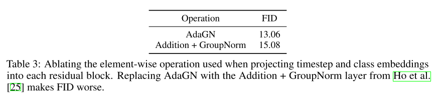
3.1 Adaptive Group Normalization
Adaptive Group Normalization(AdaGN)은 timestep과 class embedding을 각 residual block에 group normalization operation이후 넣게된다. 이 과정을 아래 수식으로 정리할 수 있다. 여기서 h는 residual block의 intermediate activation이고, $y=\left[y_s, y_b\right]$는 timestep과 class embedding의 linear projection이다.
$\operatorname{AdaGN}(h, y)=y_s \text { GroupNorm }(h)+y_b$
결론적으로 improved model architecture는 다음과 같다.
- Variable width with 2 residual blocks per resolution
- Multiple heads with 64 channels per head
- Attention at 32, 16 and 8 resolutions
- BigGAN residual blocks for up and downsampling
- Adaptive group normalization for injecting timestep and class embeddings into residual blocks
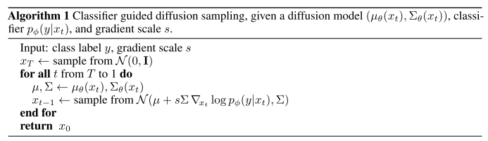
4. Classifier Guidance
Class 정보를 제공하는 것은 특정 synthetic labels image를 생성하는데 도움을 준다. Classifier $p(y \mid x)$의 gradient를 이용해 class 정보를 diffusion generator에 입력한다. 이 논문에서는 $p_\phi\left(y \mid x_t, t\right)$를 noise images $x_t$에서 학습시키고, 이것의 gradient $\nabla_{x_t} \log p_\phi\left(y \mid x_t, t\right)$를 class guidance로 사용한다.
4.1 Conditional Reverse Noising Process
Unconditional reverse noising process $p_\theta\left(x_t \mid x_{t+1}\right)$로 부터 label y에 대한 condition을 주는 수식은 아래와 같다. $Z$는 normalizing constant이다.
$p_{\theta, \phi}\left(x_t \mid x_{t+1}, y\right)=Z p_\theta\left(x_t \mid x_{t+1}\right) p_\phi\left(y \mid x_t\right)$
Diffusion model은 아래 수식을 통해 이전 timestep의 image를 생성한다.
$\begin{aligned}p_\theta\left(x_t \mid x_{t+1}\right) & =\mathcal{N}(\mu, \Sigma) \\log p_\theta\left(x_t \mid x_{t+1}\right) & =-\frac{1}{2}\left(x_t-\mu\right)^T \Sigma^{-1}\left(x_t-\mu\right)+C\end{aligned}$
limit of infinite diffusion steps($\left|\Sigma\right| \rightarrow0$) 가정에서 $\log_\phi p\left(y \mid x_t\right)$은 $\Sigma^{-1}$에 비해 low curvature를 갖는다. 이 경우 $\log_\phi p\left(y \mid x_t\right)$를 taylor expansion을 사용해 아래와 같이 기술 할 수 있다. 여기서 $g=\left.\nabla_{x_t} \log p_\phi\left(y \mid x_t\right)\right|_ {x_t=\mu}$이다.
$\begin{aligned}\log p_\phi\left(y \mid x_t\right) & \left.\approx \log p_\phi\left(y \mid x_t\right)\right|_ {x_t=\mu}+\left.\left(x_t-\mu\right) \nabla_{x_t} \log p_\phi\left(y \mid x_t\right)\right|_ {x_t=\mu} \& =\left(x_t-\mu\right) g+C_1\end{aligned}$
위 수식을 이용해 generation process를 아래 수식처럼 다시 기술할 수 있다.
$\begin{aligned}\log \left(p_\theta\left(x_t \mid x_{t+1}\right) p_\phi\left(y \mid x_t\right)\right) & \approx-\frac{1}{2}\left(x_t-\mu\right)^T \Sigma^{-1}\left(x_t-\mu\right)+\left(x_t-\mu\right) g+C_2 \& =-\frac{1}{2}\left(x_t-\mu-\Sigma g\right)^T \Sigma^{-1}\left(x_t-\mu-\Sigma g\right)+\frac{1}{2} g^T \Sigma g+C_2 \& =-\frac{1}{2}\left(x_t-\mu-\Sigma g\right)^T \Sigma^{-1}\left(x_t-\mu-\Sigma g\right)+C_3 \& =\log p(z)+C_4, z \sim \mathcal{N}(\mu+\Sigma g, \Sigma)\end{aligned}$
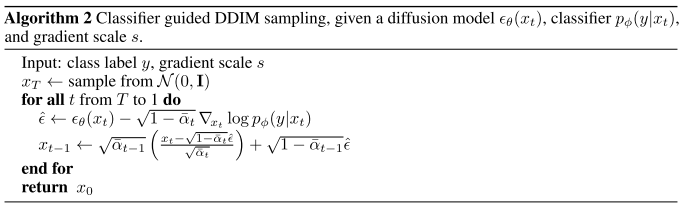
4.2 Conditional Sampling for DDIM
위의 conditional sampling수식은 stochastic diffusion sampling에서만 사용이 가능하고, DDIM과 같은 deterministic sampling methods에서는 사용할 수 없다. 이를 극복하기 위해 score-based conditioning trick을 적용한다. 그 결과로 아래 수식을 이용할 수 있다.
$\nabla_{x_t} \log p_\theta\left(x_t\right)=-\frac{1}{\sqrt{1-\bar{\alpha}_ t}} \epsilon_\theta\left(x_t\right)$
위 수식을 $p\left(x_t\right) p\left(y \mid x_t\right)$에 적용하면 아래와 같다.
$\begin{aligned}\nabla_{x_t} \log \left(p_\theta\left(x_t\right) p_\phi\left(y \mid x_t\right)\right) & =\nabla_{x_t} \log p_\theta\left(x_t\right)+\nabla_{x_t} \log p_\phi\left(y \mid x_t\right) \& =-\frac{1}{\sqrt{1-\bar{\alpha}_ t}} \epsilon_\theta\left(x_t\right)+\nabla_{x_t} \log p_\phi\left(y \mid x_t\right)\end{aligned}$
ch최종적으로 아래 수식을 기존의 $\epsilon(x_t)$대신 적용하여 DDIM과 같은 deterministic sampling methods에서도 conditional sampling이 가능하다.
$\hat{\epsilon}\left(x_t\right):=\epsilon_\theta\left(x_t\right)-\sqrt{1-\bar{\alpha}_ t} \nabla_{x_t} \log p_\phi\left(y \mid x_t\right)$
4.3 Scaling Classifier Gradients
큰 generative task에서 classifier guidance를 사용하기 위해 classification model을 ImageNet에서 학습시켰다. 모델은 UNet의 구조 중 일부를 사용했고, 데이터로 diffusion model의 noising distribution을 사용했다. Overfitting을 막기위해 random crop도 이용했다.
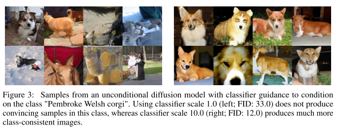
학습된 classification model을 사용할 때 scaling factor가 중요했다. Scaling factor가 1일 때는 desired class가 50%의 확률로 생성되었다. Scaling factor를 크게 적용했을 때는 아래 그림처럼 합리적인 결과를 얻을 수 있었다.
Scaling factor s는 아래 수식처럼 적용된다.
$s \cdot \nabla_x \log p(y \mid x)=\nabla_x \log \frac{1}{Z} p(y \mid x)^s$
더 큰 scaling factor를 사용하면 desired class에 더 맞는 이미지를 생성한다. 하지만 이는 생성된 이미지 diversity의 감소도 가져온다.
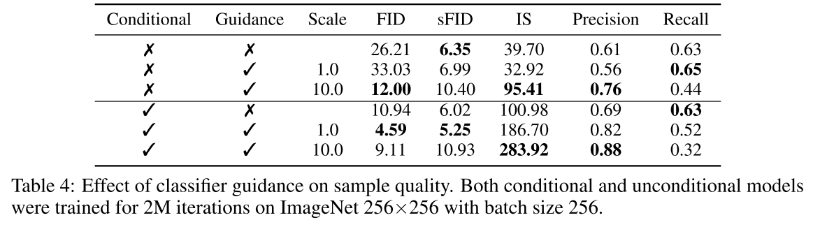
아래 표를 보면 classifier guidance가 conditional, unconditional models모두에서 성능 향상을 가져왔다. Scale에 따라서는 precision과 recall의 trade off가 확인되었다. 즉, scale을 올리면 fidelity는 상승하지만 diversity는 감소한다는 것이다.
5. Results
성능 확인을 위해 diffusion model은 3개 클래스(bedrooms, horse and cat)의 LSUN dataset을 학습시켰다. Classifier guidance로는 128, 256, 512 resolution의 ImageNet을 학습시켰다.
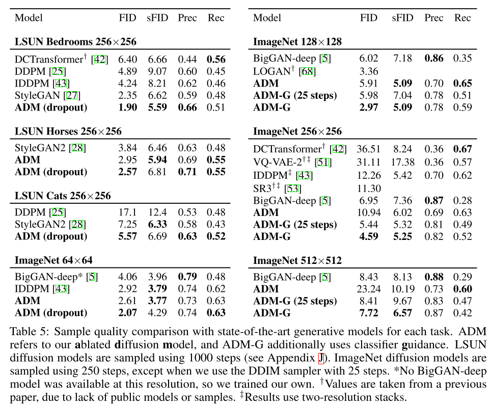
5.1 State-of-the-art Image Synthesis
이 논문의 diffusion model은 대부분의 task에서 SOTA를 찍었고, 큰 resolution의 이미지 생성에서도 좋은 성능을 보였다.
6. Related Work
생략
7. Limitations and Future Work
Diffusion model이 GAN과 비교해서 문제점은 이미지를 생성하는데 여러번 모델을 거쳐야하고, 이로 인해 시간이 오래걸린다는 것이다. 이런 점을 해결하기 위해서 Luhman and Luhman은 바로 DDIM sampling process를 single step으로하는 연구가 있다.
Proposed classifier guidance는 labeled dataset에 한정되어 있다. In the future, unlabeled data에 대해 clustering samples를 사용하여 synthetic labels를 생성하여 이를 극복할 수 있을 것이다.
8. Conclusion
이 논문에서 보여준 diffusion model을 사용해 안정된 학습을 통해 GAN보다 더 나은 이미지를 생성했다. Classifier guidance를 통해서 class-conditional task를 unconditional image generation model을 통해 해결할 수 있었다. 그리고 Scaling factor를 조절하여 특정 class의 fidelity와 diversity를 조절할 수 있었다.
'컴퓨터비전 : CV > GAN' 카테고리의 다른 글
| [논문 리뷰] StyleGAN-NADA: CLIP-Guided Domain Adaptation of Image Generators (1) | 2023.03.04 |
|---|---|
| [논문 리뷰] StyleCLIP: Text-Driven Manipulation of StyleGAN Imagery (0) | 2023.03.04 |
| [논문 리뷰] StarGAN (1) | 2022.09.01 |
| [논문 리뷰] Unsupervised Pixel-level Domain Adaptation with GAN (0) | 2022.04.11 |

